1-Lipschitz Neural Distance Fields
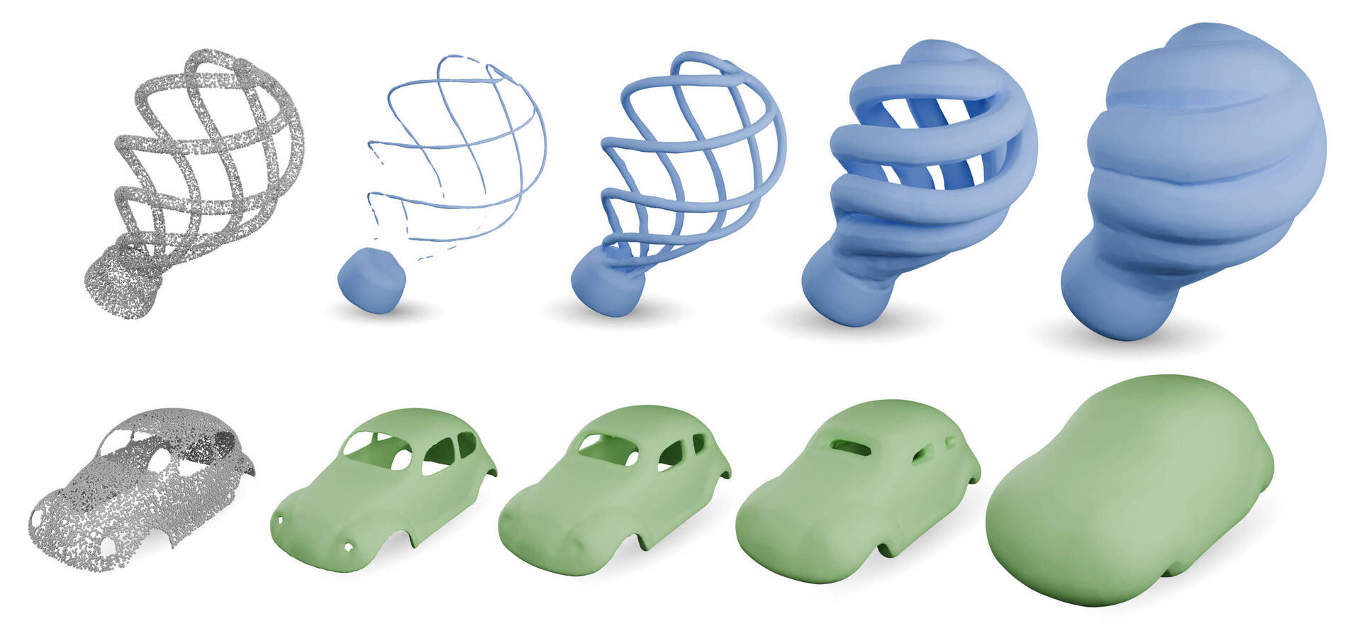
Table of contents
Signed Distance Function
This work aims at computing good quality implicit representation of implicit objects. Instead of relying on discrete structures like point clouds, voxel grid or meshes to represent a geometrical object, those representations define surface and curves as the level set (usually the zero level set) of some function. Among the infinity of continuous functions that can implicitly represent a given an object $\Omega \subset \mathbb{R}^n$, the one that best preserves the properties of $\Omega$ far from its zero level set is the Signed Distance Function (SDF) of $\Omega$, which is defined as:
$$S_\Omega(x) = \left[\mathbb{1}{\mathbb{R}^n \backslash \Omega}(x) - \mathbb{1}{\Omega}(x) \right] \min_{p \in \partial \Omega} ||x - p||$$
where $\partial \Omega$ is the boundary of $\Omega$.
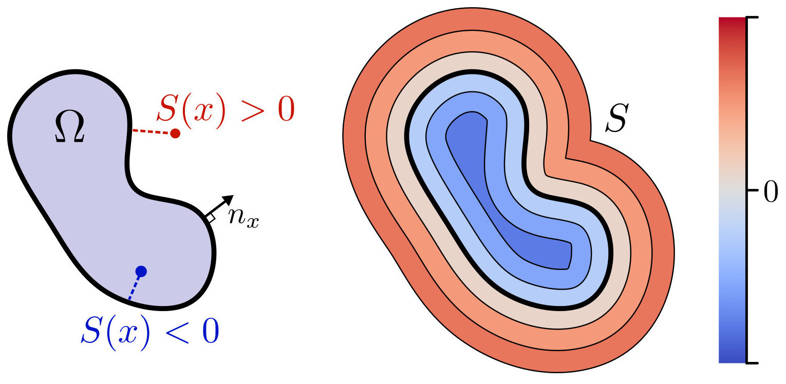
Figure 1. An implicit surface is defined as the level set of some continuous function. Among all possible functions, the signed distance function best preserves geometrical properties far from the surface.
An important property of SDFs is that they satisfy an Eikonal equation:
$$\left{ \begin{array}{lll} ||\nabla S(x)|| &= 1 \quad &\forall x \in \mathbb{R}^n \ S(x) &= 0 \quad &\forall x \in \partial \Omega \ \nabla S(x) &= n(x) \quad &\forall x \in \partial \Omega \end{array} \right.$$
Having access to the SDF of an object allows for easy geometrical queries and efficient rendering via ray marching. For example, the projection onto the surface of $\Omega$ can be defined as:
$$\pi_\Omega(x) = x - S_\Omega(x) \nabla S_\Omega(x).$$
Neural Distance Fields
The problem with SDFs is that they are difficult to compute. For simple shapes, they may be computed in closed form (see this webpage by Inigo Quilez that lists many of them), but they quickly become intractable when the objects grows in complexity. This is why there is an ongoing effort to compute good approximations of SDFs. In particular, the recent domain of neural distance fields proposes to use deep learning to solve this problem. The idea here is to define a neural network $f_\theta : \mathbb{R}^n \rightarrow \mathbb{R}$ that will approximate the SDF. However, this approach has two critical limitations:
The neural function is usually trained in a regression setting by fitting the correct values on a dataset of points where the true distance function is known. This implies that the input geometry needs to already be known very precisely for such a dataset to be extracted. In other words, one usually need to know the SDF to compute an approximation of the SDF…
The final neural network is an approximation of the SDF, which means that it does not exactly satisfy the Eikonal equation. In practice, this means that the norm of its gradient can be a little less or a little more than 1, even with regularization in the loss function:
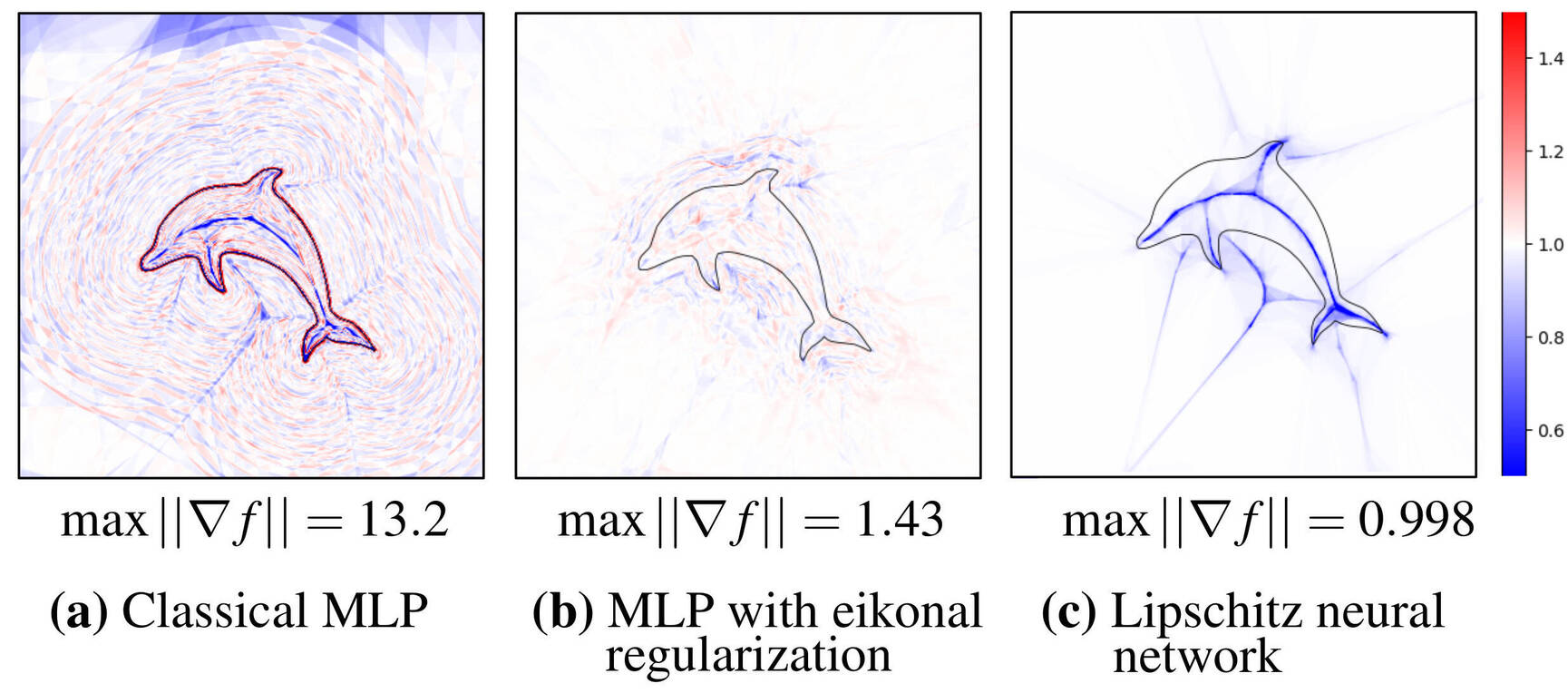
Figure 2. Plot of a the gradient norm of neural distance fields on a simple 2D dolphin silhouette. While minimizing the eikonal loss stabilizes the gradient norm, only a Lipschitz network guarantees a unit bound.
Why is this second point a problem? If the gradient exceeds unit norm, there is a risk that the function $f_\theta$ overestimates the true distance, which breaks the validity of geometrical queries like projection on the surface (Fig 3. center). If the implicit function always underestimates the distance (Fig 3. right), iterating the projection process will always yield the correct result at the cost of more computation time.
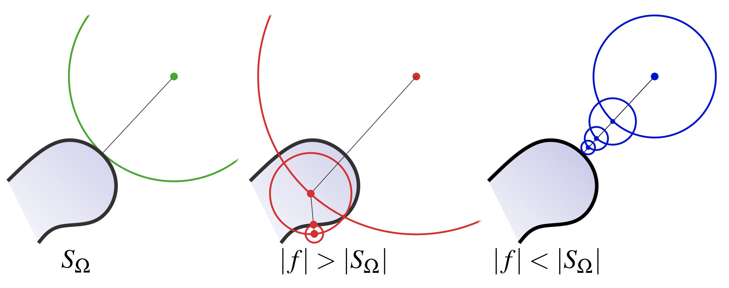
Figure 3. Closest point query on an implicit surface. Underestimating the true distance is a necessary condition for the validity of the query.
In summary, it is desirable that the neural function always underestimate the true distance. In mathematical terms, this boils down to requiring $f_\theta$ to be 1-Lipschitz, that is:
$$|f_\theta(a) - f_\theta(b)| \leqslant ||b-a|| \quad \forall a,b \in \mathbb{R}^n$$
Our method
Our method aims at building a neural distance field that is guaranteed to preserve geometrical properties far from the zero level set. In particular, we use a $1$-Lipschitz neural network so that the Lipschitz constraint will be satisfied by construction. On top of this architecture, we minimize a loss that does not need to know the ground truth distance, thus transforming the usual regression problem in a classification problem. Our method is summarized by this diagram:
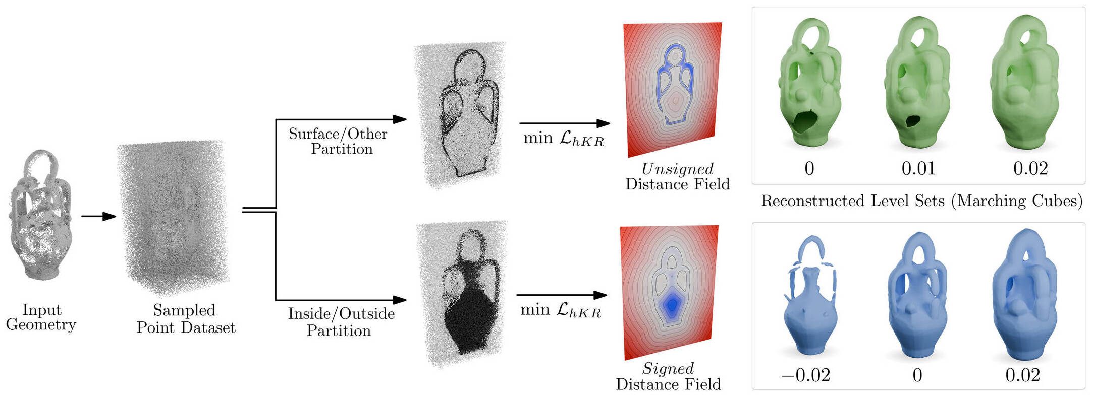
Figure 4. Given an input geometry in the form of an oriented point cloud or a triangle soup, we uniformly sample points in a domain containing the desired geometry. Defining negative samples as points of the geometry and positive samples everywhere else yields an unsigned distance field when minimizing the hKR loss. On the other hand, partitioning samples as inside or outside the shape leads to an approximation of the signed distance function of the object.
Step 1: Sampling
Our method takes as input any oriented geometry $\Omega$. This includes point cloud with normals, triangle soups and surface meshes. The first step is to extract a dataset from the input geometry. We define a domain $D \subset \mathbb{R}^n$ as a loose axis-aligned bounding box of $\Omega$ and sample it uniformly.
Step 2: Separating the interior and the exterior
The second step is to compute labels $y(x) \in {-1,1}$ for each sampled point $x$. These labels will indicate if the given point is inside or outside of $\Omega$. We propose to use the Generalized Winding Number as proposed by Baril et al. and implemented in libigl. Intuitively, the winding number $w_\Omega$ of a surface $\partial \Omega$ at point $x$ is the sum of signed solid angles between $x$ and surface patches on $\partial \Omega$. For a closed smooth manifold, the values amounts at how many times the surface “winds around” $x$, yielding an integer value. When computed on imperfect geometries, $w_\Omega$ becomes a continuous function (Fig.5). Through careful thresholding, it is still possible to determine points that are inside or outside the shape with high confidence.
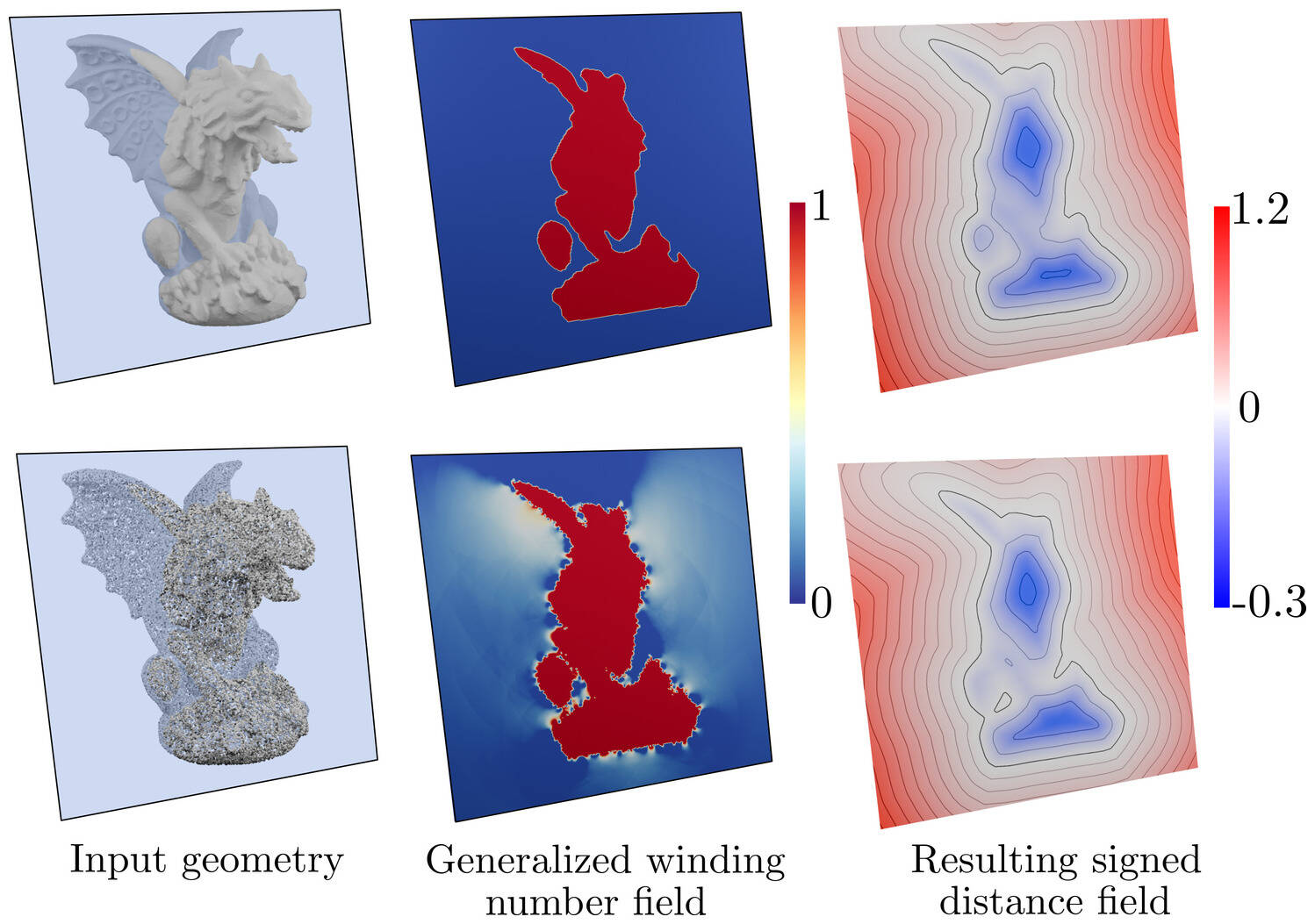
Figure 5. The generalized winding number is a robust way of knowing whether a point is inside or outside some geometrical object. For a clean manifold mesh (top row), the GWN takes integer values and classifies the inside from the outside. For imperfect geometries like oriented point clouds (bottom), the GWN is a continuous function that can be thresholded to recover the inside/outside partition.
Alternatively, one can define $y=-1$ for points on the surface of $\Omega$ and $y=1$ everywhere else. In the end, this will result in an unsigned distance field of the boundary. Doing this also extends our method to open surfaces or curves.
Step 3: Training a 1-Lipschitz network
Once the labels $y$ have been computed, we define some $1$-Lipschitz architecture to approximate the SDF. $1$-Lipschitz neural networks have been extensively studied in theoretical deep learning for their robustness to adversarial attacks and overfitting. Several architectures that are Lipschitz by construction were designed throughout the years. We use the architecture proposed by Araujo et al., although any Lipschitz architecture can be used.
On top of the Lipschitz network, we propose to minimize the hinge-Kantorovitch-Rubinstein (hKR) loss. This binary classification loss was first proposed by Serrurier et al.. For binary labels $y \in \{-1,1\}$, hyperparameters $\lambda>0$ and $m>0$ and density function $\rho(x)$ over $D$, the hKR loss is the sum of two terms:
$$\mathcal{L}{hKR} = \mathcal{L}{KR} + \lambda \mathcal{L}_{hinge}^m$$
defined as:
$$\mathcal{L}{KR}(f\theta,y) = \int_D -yf_\theta(x) \, \rho(x) dx$$ $$\mathcal{L}{hinge}^m(f\theta,y) = \int_D \max\left(0, m-yf_\theta(x)\right),\rho(x)dx.$$
We show in the paper that, under mild assumptions on $\rho$, the minimizer of the hKR loss over all possible $1$-Lipschitz functions is the SDF of $\Omega$ up to an error that is bounded by $m$. This means that minimizing the hKR loss will lead to a very good approximation of the SDF.
Gallery of results
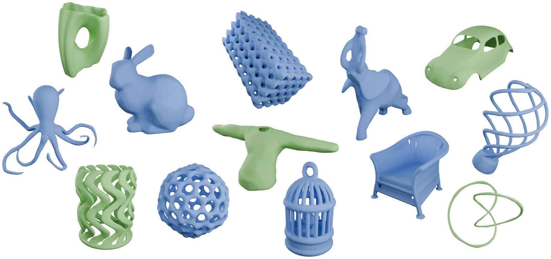
Figure 6. Surface extracted from the zero level set of a 1-Lipschitz network trained with our method. Blue surface correspond to signed distance fields while green ones are unsigned.
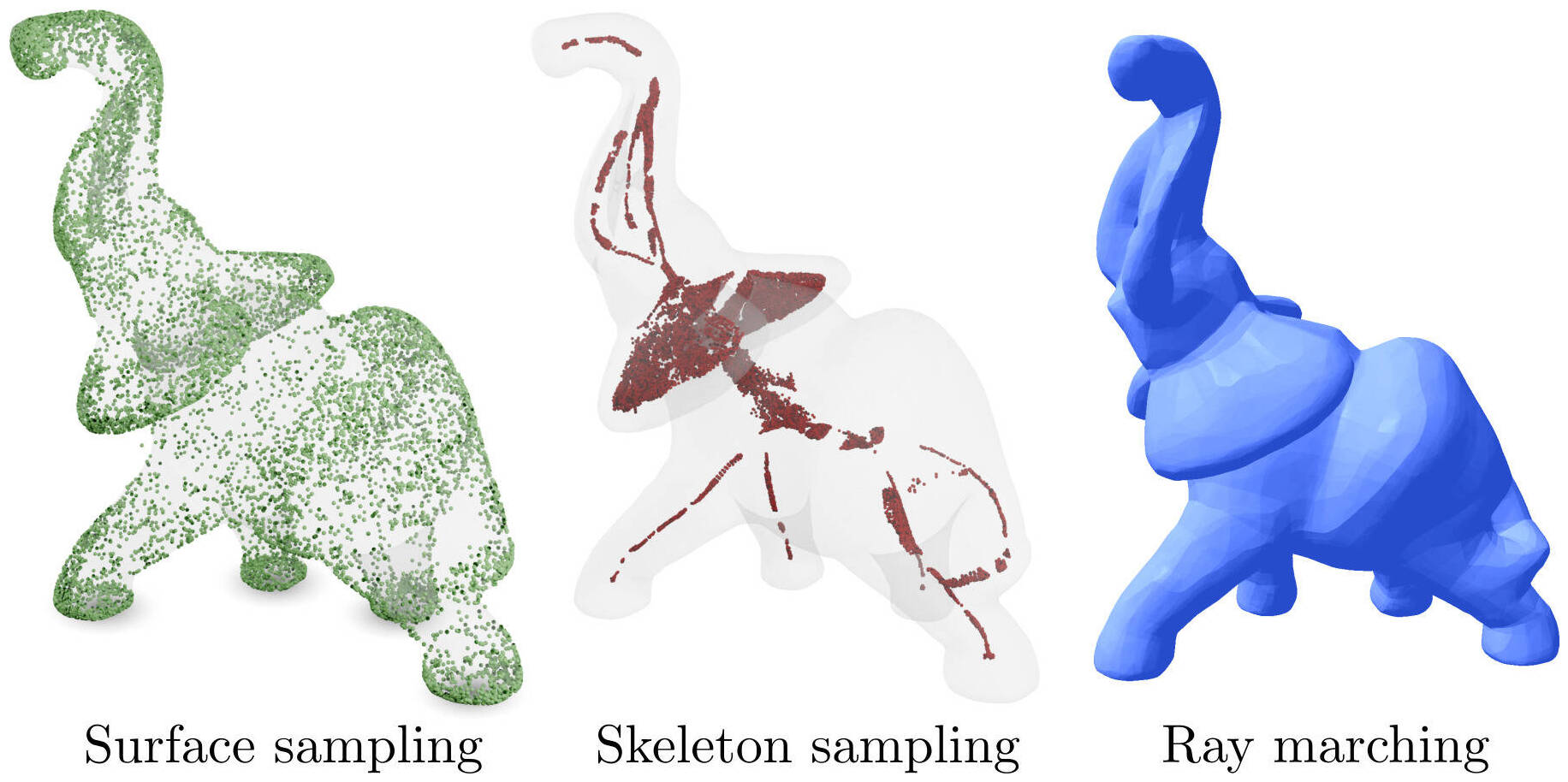
Figure 7. Robust geometrical queries performed on a Lipschitz neural implicit representation of the elephant model.
Talk video
BibTeX
@inproceedings{coiffier20241,
  title={1-Lipschitz Neural Distance Fields},
  author={Coiffier, Guillaume and B{\'e}thune, Louis},
  booktitle={COMPUTER GRAPHICS forum},
  volume={43},
  number={5},
  year={2024}
}